
In this article
 Introduction
- What are Residuals?
- Regression residual
- Residual plots
- Analysis of the residual plots
- Correlation
- Calculating the Correlation using Pearson’s correlation coefficient
- Residuals and Correlation in Regression Analysis
- Common Pitfalls in Interpreting Residuals and Correlation
- Applications of Residuals and Correlation
- Conclusion
- Sample Examples
- FAQs
Introduction
The concepts of Residuals and correlation are very important and widely used statistics terms that are related to linear regression. Linear regression is a method of analysis which is used to predict a dependent variable based on the value of an independent variable.
The regression line is the best way to represent data in a scatter plot.
An estimate of the line that depicts the actual, but the unidentified, linear connection between the two variables is called a regression line. When the value of the explanatory variable is known, the regression line’s equation is used to predict the value of the response variable.
The correlation coefficient and the residuals are some of the important technical measurements that are related to the regression line of a data.
What are Residuals?
Definition: The difference between the observed value and the mean value that a model predicts for each observation are residuals.
Every observation will have a residual in a regression line.In statistical modeling, the regression line model is used to calculate the residuals.The vertical distance from the observation to the regression line is the residual.The observations above the line would be considered positive residuals and similarly, the observations below the line would be negative residuals. We can say that the sum of the fit and residual would be the whole data.
Regression residual
Residual,
The difference between a data point’s actual value and the value that the regression line would have predicted for that identical data point is known as the residual.
Therefore, Residual is the value obtained from the difference of the actual and the predicted values.
The regression line is represented by and the actual value would be the value on the respective scale.
Hence, the formula to calculate residual for an observation is:

The sum of the residuals is always 0, i.e., .
And the mean of the residuals is also 0, i.e., .
- Calculating the residual for an observation
1. Compute the predicted value for the point to be calculated.
2. Calculate the difference using the formula.
Residual plots
They are a visual representation that is used to validate the regression models.
The residual plots have the independent variables on the x-axis and the calculated residual values on the y-axis.
Analysis of the residual plots
We can analyze the residual plots and if they show characteristics of a good residual plot, we can validate the linear regression model of the same data.
A good residual plot has the following characteristics:
- The residuals are independent and normally distributed
As we move along the x-axis if we do not see any pattern, then it would mean that the residuals are independent.
And if we project the values onto the y-axis, it should show a normally distributed curve.
- It has a low density of points far from the origin compared to a high density of points nearby.
- It is symmetric about the origin.
Correlation
Definition: A statistical metric known as correlation describes how closely two variables are connected linearly. It’s a typical technique for expressing straightforward connections without explicitly stating cause and consequence.
There are four types of correlation:
- Positive correlation: The positive linear correlation is when the variables on both the axes i.e., the x-axis and y-axis simultaneously increase thus resulting in the regression line having an upward slope.
- Negative correlation: The negative linear correlation is when either one of the variables decreases as the other increases, therefore resulting in a downward slope of the regression line.
- Non-linear correlation: There is a defined relationship between the two variables but the relationship is not linear.
- No-correlation: The two variables do not have any visible or viable relation or pattern detected.
Calculating the Correlation using Pearson’s correlation coefficient
Statistics defines Pearson correlation coefficient, often known as Pearson’s correlation coefficient or Pearson’s r, as the assessment of the strength of the link and association between two variables.
Pearson’s correlation coefficient formula:

Where:
= the number of pairs of scores.
= the sum of the products of paired scores.
= the sum of x scores.
= the sum of y scores.
= the sum of squared x scores.
= the sum of squared y scores.
Residuals and Correlation in Regression Analysis
- Residuals and Correlation in Linear Regression
The correlation coefficient is used find how strong the relationship is between the variables and .
The formula used to find the coefficient relation in linear regression

is the mean of .
is the mean of .
is the standard deviation of.
is the standard deviation of.
is the number of observations.
The correlation coefficient always lies between 1 and -1. If the value is closer to 0 the relationship is weaker and if it’s between 0.5 and 1, or -0.5 and -1 the relationship between the variables is strong.
- Residuals in Nonlinear Regression
The residuals are calculated the same way as in the linear regression i.e., the perpendicular distance between the actual and the predicted values.
- Residuals in Time Series Analysis
The residuals between the fitted values and the observed and are defined as:

Common Pitfalls in Interpreting Residuals and Correlation
- Correlation can be used only when there is a relation that is linear. A linear relationship is what the correlation coefficient seeks. As a result, it may be mistaken when two variables actually have a link, but that relationship is nonlinear.
- All observations are supposed to be independent of one another for the purposes of correlation analysis. As a result, it shouldn’t be applied when there are several observations of a single individual in the data.
- Only data on a continuous scale are appropriate for linear correlation analysis. When one or both variables have been assessed using an ordinal scale, it should not be utilized.
- We also cannot see a correlation when there is between the variable and one of its elements (components).
- We have to avoid multicollinearity. Multicollinearity is the term used to describe the relationship that develops between two or more predictor variables. This is undesirable since it adds redundancy to the model. Because the coefficient matrix
cannot reach full Rank in this situation, the least squares optimization technique is impacted.
- Another common mistake is heteroscedasticity, which is the Non-Constant Variance of Error Terms. To learn more about this, we may plot the residuals (often in a Standardized format) against the Predicted Values.
Applications of Residuals and Correlation
- Business leaders may make more meaningful predictions based on trends in data with the help of correlation and regression analysis. Through the use of this approach, company operations may be enhanced as well as management, customer experience initiatives, and performance can be guided appropriately.
- Correlation and residuals can be used in any relations between activities and their impacts such as height and weight, time spent exercising and body fat, abuse of substance and intelligence, temperature and amount of electricity used etc.
Conclusion
In this article, we learnt about how residuals and correlations are a very important part of the analysis of linear regression and how we can statistically use them to find the probable values from the observed values. We learnt about the different types of correlation, the Pearson’s correlation coefficient and how correlation can be used in linear regression. They are important tools which are used to estimate values in many real-life analyses.
Sample Examples
Example 1: Find the correlation coefficient for the given data set.
 | 2 | 4 | 6 | 8 | 10 |
 | 0.6 | 1.0 | 0.4 | 0.4 | 2.0 |
Solution 1:
We need to find the means of and .


Now we find the standard deviations and.


Now we use the formula to calculate the correlation coefficient and substitute the values calculated.

The correlation coefficient is 0.647
Example 2: Find the residuals for the data given and make a scatterplot with the residual values. (Residual plot)
| 0 | 2 | 4 | 6 | 8 |
| Actual | 0.6 | 1.0 | 0.4 | 0.4 | 2.0 |
| Predicted | 0.543 | 0.967 | 0.698 | 0.836 | 0.942 |
Solution 2:
We use the formula.
Therefore, the residuals for each observation would be
| 0 | 2 | 4 | 6 | 8 |
 | 0.057 | 0.033 | -0.298 | -0.436 | 1.058 |
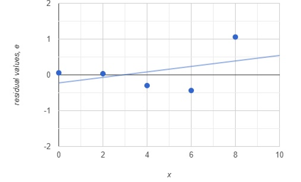
Plotting the calculated values against we get the above plot.
Example 3: For a linear fit , calculate the residual for the observation (40,82.1).
Solution 3:
First, we find the value of which is
The given value of is 82.1.
Using the formula,we get the value of to be
Therefore, the residual value is 1.1
Example 4: For a linear regression find the residuals for the observations (1,2) and (6,4).
Solution 4:
First, we find the value of which is for the first point and
The given value ofis 2 for the first observation and 4 for the second one.
Using the formula ,
| |
| Observation 1 | -7 |
| Observation 2 | -25 |
Example 5: Find the residuals of the yellow observation and the green observation from the graph given below:
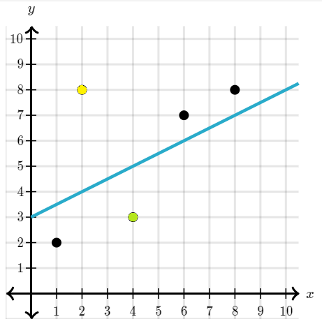
Solution 5:
Using the formula
For the yellow observation the value of is 8 and the value ofis 4.
Therefore, is 4.
For the green observation the value of is 3 and the value of is 5.
Therefore, is -2.
FAQs
1. What is the normal distribution?
Ans: An example of a continuous probability distribution is the normal distribution, in which the majority of data points cluster in the middle of the range while the remaining ones taper off symmetrically toward either extreme.
2. What is an independent variable?
Ans: The cause in a study is the independent variable. Its value is unaffected by the other research factors.
3. What is a scatter plot?
Ans: The graphs that show the association between two variables in a data collection are called scatter plots. It displays data points either on a Cartesian system or a two-dimensional plane. The X-axis is used to represent the independent variable or characteristic, while the Y-axis is used to plot the dependent variable.
4. What is linear regression?
Ans: A variable’s value can be predicted using linear regression analysis based on the value of another variable. The dependent variable is the one you want to be able to forecast. The independent variable is the one you’re using to make a prediction about the value of the other variable.
5. What is the time series?
Ans: A time series is a group of observations of clearly defined data points produced over time via repeated measurements.
References
Whitley, E., & Ball, J. (2002). Statistics review 2: Samples and populations. Critical Care, 6(2), 1-6.
Cox, D. R., & Snell, E. J. (1968). A general definition of residuals. Journal of the Royal Statistical Society: Series B (Methodological), 30(2), 248-265.Zou, K. H., Tuncali, K., & Silverman, S. G. (2003). Correlation and simple linear regression. Radiology, 227(3), 617-628.
Mar 11, 2025
Was this helpful?


