
In this article
Introduction
A chi-square test is a statistical test used to compare observed results with expected results. It is the analysis of the data based on the observations of a random set of variables and is used to compare sets of statistical data.
Chi-square tests are used in hypothesis testing where a condition can be true, and it is tested afterwards. The tests are used to estimate the irregularities between the actual results and the expected results using the number of variables and the size of the samples.
The test is used to estimate how likely the observations made would be, by considering the null hypothesis to be true.
The null hypothesis is a hypothesis in which the sample observations result from the chance. The null hypothesis is a kind of hypothesis which explains the population parameter whose purpose is to test the validity of the given experimental data.
Understanding the Chi-Square
- Chi-square distribution
Considering the null hypothesis to be true, the sampling distribution of the test statistic is called the chi-square distribution.
The test is used to determine if there is a significant difference between the observed frequencies and the normal frequencies. It gives the probability of independent variables.
- The degree of freedom
It is calculated by the formula:

Where:
is the degree of freedom.

is the number of columns.
- The P-value in statistics
P is the value for probability and the chi-square is used to calculate it.
It defines the probability of getting a result that is either the same or more extreme than the other actual observations. The P-value represents the probability of occurrence of the given event.
The hypothesis interpretation and the value of P relation is as follows:
If then the hypothesis is rejected.
If then the hypothesis is accepted.
Applications of the Chi-Square test
The Chi-square test which is also called the 
- Homogeneity: To determine if two populations with uncertain distributions share the same distribution, use the homogeneity test. In this instance, two distinct populations will each get one qualitative survey question or experiment.
The alternate and null hypotheses are:
: the populations follow the same distribution.
: the population has different distributions.
- Goodness-of-fit: Use the goodness-of-fit test to ascertain if a population with an unknown distribution matches a known distribution. In this case, there will only be one qualitative survey question or one experiment’s findings from one demographic. In order to evaluate if a population is uniform (all outcomes occur with the same frequency), normal, or identical to another population with a known distribution, the Goodness-of-Fit test is widely employed.The alternate and null hypotheses are:
: the population fits the given distribution.
: the population does not fit the given distribution.
- Independence: To determine if two variables (factors) are independent or dependent, use the independence test. In this instance, a contingency table will be built along with two qualitative survey questions or experiments. The objective is to determine if the two variables are connected or unrelated (dependent).
The alternate and null hypotheses are:
: the two variables are independent.
: the two variables are dependent.
Properties
Some of the major properties of the chi-square test are:
- The chi-square distribution curve approaches the normal distribution when the degree of freedom increases.
- The number of degrees of freedom is equal to the mean distribution.
- Two times the number of degrees of freedom is equal to the variance.
Formula
The formula for the chi-square test is to check the difference between the observed value and expected value.
The formula is:
Where,
is the observed value,
is the expected value.
Steps to use Chi-Square Test
- Define the hypothesis, i.e., find the right definition we want to use forandof the data.
- Calculate the expected frequency value using the formula:
- Calculate for each cell.
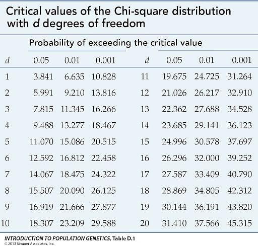
- Now we have to determine the critical statistics and we use the formula of degree of freedom and then choose an appropriate alpha level in the critical values of chi-square distribution table with .
The table is as follows:
If the obtained value of
Limitations of the Chi-Square test
- Only the relationship between two variables can be determined using the chi-square. It does not follow that there must be a causal connection between two variables.
- To begin with, the chi-square test is very sensitive to sample size. When a big enough sample is employed, even small corrections and connections might seem statistically significant.
- The Chi-square statistic is only applicable to numerical data. They are not applicable to information with percentages, proportions, means, or other statistical components.
Conclusion
The chi-square test is a very important topic in statistical analysis of random data sets and is used in day-to-day analysis of expected values. We learnt how the chi-squared distribution works and how to find the related values. We also learnt how the chi-square value and the critical value are related.
Solved Examples
Example 1: Calculate the Chi-Square value of the following data of cars by each family in the area using the data given in the table below.
| Number of cars |  |  |
| One car | 25 | 20.4 |
| Two cars | 13 | 11 |
| Three cars | 7 | 5.9 |
| Total | 45 |
Solution 1:
To find the chi-square let us use the formula
Finding for each category we get
| One car | 1.04 |
| Two cars | 0.36 |
| Three cars | 0.21 |
Hence
The chi-square value is 1.61.
Example 2: The number of corn dogs sold during a carnival to men, women and children and the percentage of the total corndogs bought are as follows. Find the Chi-square value.
| Category | | Percentages |
| Men | 64 | 40 |
| Women | 45 | 20 |
| Children | 50 | 20 |
| Total | 159 |
Solution 2:
First, we need to find the expected value for each category.
| Category | |
| Men |  |
| Women |  |
| Children | |
Now let us use the formula to calculate the value of for each category.
| Category |  |
| Men | 0.002 |
| Women | 5.439 |
| Children | 10.416 |
Now we find the sum of the calculated values to get 
Hence,
Example 3: The number of times (in million) the songs by different artists has been streamed is as follows. Find the Chi-Square.
| Artists | | |
| Drake | 13 | 11 |
| Travis Scott | 25 | 22 |
Solution 3:
To find the chi-square let us use the formula
Findingfor each artist we get:
| Artists | |
| Drake | 0.36 |
| Travis Scott | 0.41 |
Hence
The chi-square value is 0.77.
Example 4: The sample for the voting of prom queen are given as follows. Prom queen 1 and 2 are two girls who were nominated for it.
| Prom queen 1 | Prom queen 2 | Total | |
| Male | 10 | 12 | 22 |
| Female | 14 | 6 | 20 |
| Total | 24 | 18 | 42 |
Find out if gender has anything to do with the prom queen preference.
Solution 4:
We first define a hypothesis.
: There is no link between gender and prom queen preference.
: There is a link between gender and prom queen preference.
Now lets calculate the expected values for each cell using .
| Prom queen 1 | Prom queen 2 | Total | |
| Male | 12.57 | 9.42 | 22 |
| Female | 11.42 | 8.57 | 20 |
| Total | 24 | 18 | 42 |
Now we need to calculate for each cell.
| Prom queen 1 | Prom queen 2 | |
| Male | 0.525 | 0.706 |
| Female | 0.583 | 0.770 |
Now to calculate
Hence, the value of
Let us find the value of which is:


We use the value to determine the critical value using from the table.
We get the critical value to be 3.841.
We can see that our value (2.584) is lesser than the obtained critical value (3.841).
Hence, we can accept our null hypothesis.
Example 5: In a survey of cars, a sample of the study of the number of Audi cars and Jeep cars in two cities, city1 and city2 are as follows. Find the chi-square and see if there is a link between the cities and the type of cars used.
| City1 | City2 | Total | |
| Audi | 45 | 60 | 105 |
| Jeep | 50 | 40 | 90 |
| Total | 95 | 100 | 195 |
Solution 5:
We first define a hypothesis.
: There is no link between gender and prom queen preference.
: There is a link between gender and prom queen preference.
Now let’s calculate the expected values for each cell using
| City1 | City2 | Total | |
| Audi | 51.15 | 53.85 | 105 |
| Jeep | 43.85 | 46.15 | 90 |
| Total | 95 | 100 | 195 |
Now we need to calculate for each cell.
| City1 | City2 | |
| Audi | 0.739 | 0.702 |
| Jeep | 0.863 | 0.820 |
Now to calculate
Hence, the value of
Let us find the value of which is:
We use the value to determine the critical value using from the table.
We get the critical value to be 3.841.
We can see that our value (3.124) is lesser than the obtained critical value (3.841).
Hence, we can accept our null hypothesis.
FAQs
1. What is a preferred and advisable Chi-square value?
Ans: The Chi-square value of 5 is considered to be good. The anticipated frequency must be at least five for a chi-square method to be reliable.
2. What are critical values in statistics?
Ans: Critical value in statistics is a cut-off value that is compared with a test statistic in hypothesis testing to check whether the null hypothesis should be rejected or not.
3. What does it mean when the calculated chi-value is close to the critical value?
Ans: The hypothesis needs more attention.
4. Where else is the degree of freedom used in statistics?
Ans: It is an essential idea that appears in many contexts throughout statistics including hypothesis tests, probability distributions, and linear regression.
5. What kind of statistical data is used for chi-square calculation?
Ans: The data used in calculating a chi-square statistic must be random, raw, mutually exclusive, drawn from independent variables, and drawn from a large enough sample.
References
Lancaster, H. O., & Seneta, E. (2005). Chi‐square distribution. Encyclopedia of biostatistics, 2.Wilson, E. B., & Hilferty, M. M. (1931). The distribution of chi-square. Proceedings of the National Academy of Sciences, 17(12), 684-688
Mar 10, 2025
Was this helpful?


